LaTeX stuff#
This page describes how showyourwork! parses your LaTeX manuscript (by default,
the file src/ms.tex) and uses it to build your article PDF. While you can
do just about anything you’d regularly do when writing in LaTeX, there are a
few rules and details you should be aware of controlling the generation of figures
and the inclusion of clickable margin icons, which we discuss in detail below.
Overview#
By default, the LaTeX manuscript that gets compiled into your paper PDF looks something like this:
% Define document class
\documentclass[twocolumn]{aastex631}

% Import showyourwork magic
\usepackage{showyourwork}

% Begin!
\begin{document}

% Title
\title{An open source scientific article}

% Author list
\author{First Author}

% Abstract with filler text
\begin{abstract}
    Lorem ipsum...
\end{abstract}

% Main body with filler text
\section{Introduction}
Lorem ipsum...

\end{document}
When you run showyourwork!, the workflow generates a PDF that looks something like this:
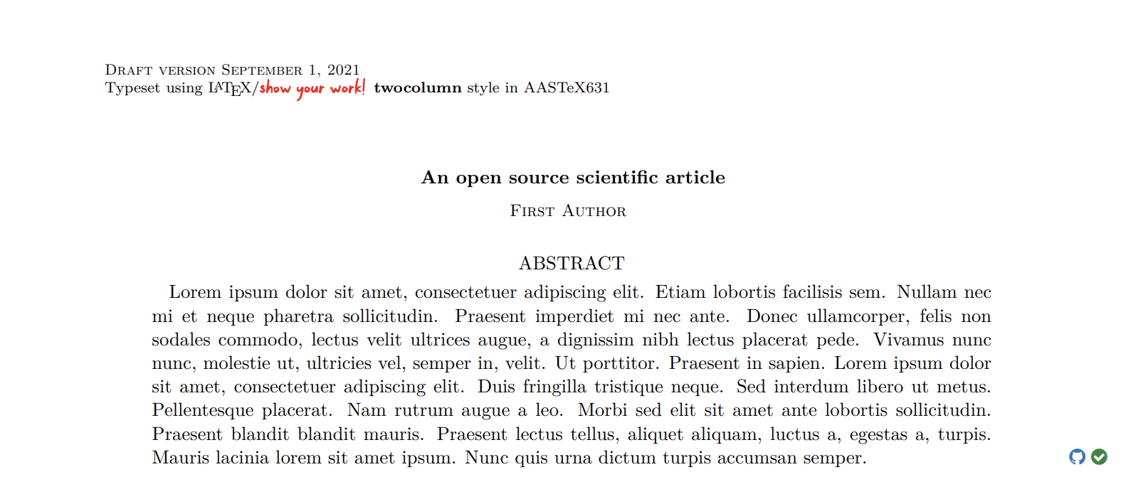
When you execute your workflow, showyourwork! dynamically embellishes the
showyourwork.sty file with all of the metadata needed to annotate the PDF
with the custom margin icons linking to the repository and the scripts that
generated the individual figures.
While most users don’t have to worry about how any of this works, it’s important to
keep in mind that this dynamically-generated style sheet redefines certain LaTeX commands under
the hood, such as the abstract and figure environments and the
includegraphics command. For instance, in order to include the
margin icons next to the abstract, showyourwork! simply patches the abstract
command to include a marginnote. If you try to compile your PDF with a standard
TeX compiler (such as pdflatex), things should work just fine (as long as
the figures have all been previously generated), but you won’t get any of the
annotations mentioned above.
The showyourwork! style sheet also defines a few useful commands, the most
important of which are the script command for specifying figure scripts
and the variable command for specifying programmatically-generated stuff
in your TeX file.
Let’s talk about those two next.
The \script command#
In a nutshell, the idea behind showyourwork! is to have users place all the
figure-generating scripts in the src/scripts directory, and the workflow
will automatically execute them when generating the article PDF.
However, it would be pretty wasteful to re-run all of the scripts every time
we build the article PDF, since many of the scripts likely haven’t changed
since the last time the article was built.
It’s therefore useful for showyourwork! to know exactly which scripts generate
which figures so it can optimize the build process.
There are different ways the user can do this, but the easiest is to
call the \script command within a figure environment, as follows:
\begin{figure}
    \begin{centering}
        \includegraphics{figures/mandelbrot.pdf}
        \caption{This is a pretty visualization of the Mandelbrot set.}
        \label{fig:mandelbrot}
        \script{mandelbrot.py}
    \end{centering}
\end{figure}
Within this figure environment, we’ve declared the figure we wish to include
(figures/mandelbrot.pdf, where the path is relative to the tex file),
the label we’ll use to reference the figure
(fig:mandlebrot), and the name of the script that generates all of the
graphics in this environment (mandelbrot.py, which is relative to
the src/scripts directory). Figure environments can only have a single
\script declaration, and must include a figure label.
Important
Previous versions of showyourwork! inferred the name of the figure
script directly from the label. This functionality is now deprecated,
and there are no longer any restrictions on the formatting of the
argument of the \label command within a figure environment.
If a figure environment does not include a \script declaration, or
if a figure is included outside of a figure environment, the user must
provide a custom Snakemake rule to generate it (see Intro to Snakemake), unless this figure
is present in the src/static directory (see below).
Otherwise, LaTeX will throw an error saying the figure can’t be found at build time.
There are certain cases in which the user may want to override the showyourwork!
functionality and provide custom rules to generate the figures. This may be the
case if a single figure environment contains multiple figures generated by
different scripts. In this case, the user should not provide a \script
declaration and instead define a rule in the Snakefile explicitly describing the
relationship between the scripts and figures (see Intro to Snakemake for more details).
There is one other use case worth mentioning: including a figure that can’t be
programmatically generated (such as a photograph, a drawing, or a manually-created diagram).
This can be done by simply placing the figure in the src/static
directory (and committing it to the repo); no \script command is necessary
within the figure environment. showyourwork! will look in the src/static
directory and, if it finds the relevant file, it will automatically copy the figure
over to the src/tex/figures directory so it can be ingested during the build.
There are a few other idiosyncrasies about this whole procedure, mostly
related to the use of the label command. Specifically, the \label
command in a figure environment should always
come after the caption and should never be inside the caption. You’ll
run into warnings or errors if you try to do one of those things (since it
messes up the way showyourwork! builds the internal tree representation
of your article). Also, it’s useful to know that showyourwork! isn’t
directly parsing your LaTeX, meaning that even if you alias your label command
and use that alias, the functionality described above will still work!
The same applies to \includegraphics calls. You can use related commands
to include your figures (like \plotone or a custom command), and things
should still work as long as \includegraphics is invoked at some point
by those functions.
The \variable command#
At the surface, the \variable command is just
an alias of the built-in \input command, which allows you to include
the content of an arbitrary file in your manuscript. This is useful for including
the contents of a dynamically-generated file containing, e.g., the value of a
variable that is output by your workflow. The main difference between \input and
\variable is that the latter explicitly marks the file as a dependency of
the manuscript in the workflow graph, which automatically generates the file if
it is missing and re-builds the article whenever the script or rule that generates
that file is modified.
Note that users could instead use \input and manually include the
file as a dependency in the showyourwork.yml config file,
but errors may occur during the initial
pre-processing step if the file does not already exist. A workaround for this is
to nest the \input command in a \IfFileExists{}{} conditional, but we
simply recommend you use the \variable command instead for
including programmatically-generated files!
When using the \variable command, you probably want to also define a rule
in the Snakefile to generate the file. For example, say you want to include
the contents of the file answer.txt in your TeX file:
ms.tex#The answer to the ultimate question of life, the universe, and everything
is \variable{output/answer.txt}.
If this file is generated by running the script deep_thought.py, you can
inform the workflow about it by adding the following rule to your Snakefile:
Snakefile#rule compute_answer:
input:
"src/data/universe.dat"
output:
"src/tex/output/answer.txt"
script:
"src/scripts/deep_thought.py"
And that’s it – your article PDF will now update whenever anything in the input file(s) to the rule (which include the Python script itself) changes.
Finally, note that even though the command is called \variable, you can
use it to include any file containing text or arbitrary TeX commands, such
as a programmatically-generated table or even AI-generated text. We recommend
generating all of these files in the src/tex/output directory.
See Intro to Snakemake for more information.
arXiv submission#
Sometimes you may have to compile your article directly with pdflatex
or using a third-party tool that compiles LaTeX internally. This is the case
when submitting to the arXiv – you upload the source
and your PDF is compiled for you.
showyourwork! facilitates this for you via the
showyourwork tarball
command, which places all the relevant class and style files in the src/tex
directory so you can build your article PDF using a
standard LaTeX compiler. Running this command packages everything up into
a tarball, which you should be able to upload to arXiv straight away.
Custom commands#
There are a few custom commands provided by showyourwork! that you should be able to use anywhere in your texfile:
\showyourwork#
This is a command that takes no arguments and simply adds a tiny inline showyourwork! logo. Useful for bragging to your friends about your cool new toy!
\marginicon#
This command takes a single argument, which it places in the margin next
to a figure caption. This can be used to include custom margin icons or to
override the showyourwork!-generated icons. It should be included after
any calls to \caption and before any calls to \label.
\GitHubURL#
A macro that resolves to the current repository URL
(i.e., https://github.com/user/repo).
\GitHubSHA#
A macro that resolves to the current commit SHA
(i.e., 31860f2f558b05d8c941d8f73c64f5dbf5ee79db).
Reproducibility paragraph#
To explain to the readers of your article how showyourwork! operates, how they can reproduce your science, and where to find the data and scripts used, it can be useful to have a brief paragraph or appendix in your manuscript. This is also often helpful to meet the reproducibility requirement of scientific journals and make your article self-contained. Typically this will also contain the doi of the zenodo repository associated to your article.
The following is an example from the appendix E of Renzo et al. 2023 that can be adapted for your own manuscript:
This study was carried out using the reproducibility software
\href{https://github.com/showyourwork/showyourwork}{\showyourwork}
\citep{Luger2021}, which leverages continuous integration to
programmatically download the data from
\href{https://zenodo.org/}{zenodo.org}, create the figures, and
compile the manuscript. Each figure caption contains two links: one
to the dataset stored on zenodo used in the corresponding figure,
and the other to the script used to make the figure (at the commit
corresponding to the current build of the manuscript). The git
repository associated to this study is publicly available at
\url{https://github.com/mathren/CE_accretors}, and the release
v.2.1 allows anyone to re-build the entire manuscript. The datasets
are stored at \url{https://doi.org/10.5281/zenodo.7343715}, including
the template setup to recreate them using MESA (version 15140 and
the software development kit \texttt{x86\_64-linux-20.12.1}) and
the scripts used to produce the figures.
The bibliographic reference Luger2021 can be found at
Attribution .