Quickstart
Contents
Quickstart#
Install#
To get started with showyourwork!, install it using the pip command:
pip install showyourwork
You’ll also need to have the conda package manager installed, which you
can download from this url.
Setup#
To set up a blank article, simply execute the showyourwork setup command. This
command accepts one positional argument: the “slug” of the GitHub repository
for the article, which is a string in the form user/repo. For example,
to create a repository called article under the GitHub user rodluger,
run
showyourwork setup rodluger/article
This will bring up the following prompt:
Let's get you set up with a new repository. I'm going to create a folder called

    article

in the current working directory. If you haven't done this yet, please visit

    https://github.com/new

at this time and create an empty repository called

    rodluger/article
As requested, if you haven’t yet created the remote repository, go to github.com/new in your browser to create an empty repository of the same name. There’s no need to create a README, gitignore file, or LICENSE at this time, as showyourwork! will set those up for you.
Press any key to bring up the next prompt:
You didn't provide a caching service (via the --cache
command-line option), so I'm not going to set up remote caching for this repository.
The showyourwork! workflow automatically caches the results of intermediate
steps in your pipeline on Zenodo, but only if the user requests it via the --cache
option. Let’s not worry about this for
now – you can read up on how this all works at Zenodo integration.
Press any key to bring up the final prompt:
You didn't provide an Overleaf project id (via the --overleaf command-line
option), so I'm not going to set up Overleaf integration for this repository.
The workflow can also manage integration with an Overleaf project if that’s how
you prefer to write your TeX articles. To enable this, re-run showyourwork setup
with --overleaf=XXX, where XXX is the 24-character project id of a
blank Overleaf repository (you can grab this value from the URL of the project
after creating it on Overleaf). Let’s again skip this for now – read all about it
at Overleaf integration.
Finally, press any key to generate the repository. This will create a new folder
in the current working directory with the same name as your repo (article, in
the example above) and set up git tracking for it.
Build locally#
Your new repository is instantiated from a bare-bones template with the minimal
showyourwork! layout, which you can read about at Repository layout.
The first thing you might want to do is edit the main TeX file, which is located
at src/tex/ms.tex. Give it a custom title, edit the author name, and replace
some of the Lorem Ipsum placeholder text with something informative. Then,
compile the article PDF by running
showyourwork build
or, as a shorthand, just
showyourwork
in the top level of your repository. The first time you run this, showyourwork!
will set up a new conda environment and install a bunch of packages, so it
could take one or two minutes. The workflow will then build your article PDF,
which by default is saved as ms.pdf in the top level of your repository:
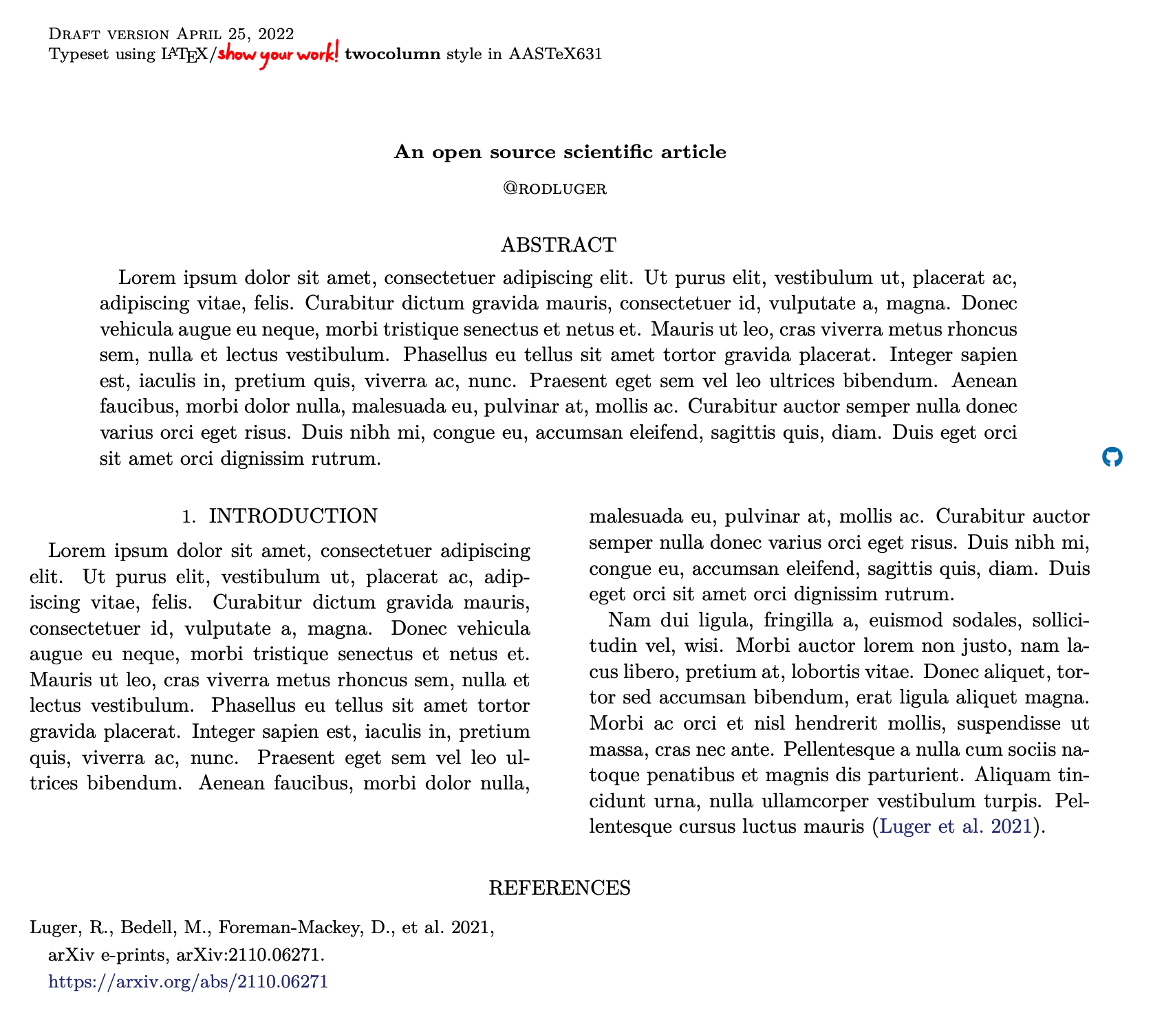
There’s not much to see – mostly placeholder text. One thing to note, though,
is the blue GitHub icon in the right margin next to the abstract: this is a
hyperlink pointing to your github repository (or, in this example, to
github.com/rodluger/article.)
Let’s turn this into a proper scientific article by adding a figure. In
showyourwork!, all figures should be programmatically generated, so we start
by creating a script to generate the figure. For simplicity, let’s create a
script random_numbers.py to generate and plot some random numbers:
import matplotlib.pyplot as plt
import numpy as np
import paths

# Generate some data
random_numbers = np.random.randn(100, 10)

# Plot and save
fig = plt.figure(figsize=(7, 6))
plt.plot(random_numbers)
plt.xlabel("x")
plt.ylabel("y")
fig.savefig(paths.figures / "random_numbers.pdf", bbox_inches="tight", dpi=300)
By default, the showyourwork! workflow expects figure scripts to be located in
(or nested under) src/scripts, so that’s where we’ll put this script.
Important
The default location for figure output (i.e., the generated .pdf figure files)
is in the src/tex/figures directory, so we need to make sure figure scripts
save their output into that folder, regardless of where the script is executed
from. The simplest way to do this is to import the
paths module, a file that is automatically included in the src/scripts
directory when you create a new article repository with showyourwork!. This
module defines a few convenient paths, like figures and data. These are instances of
pathlib.Path objects pointing to the absolute paths of various useful workflow
directories.
Now that we’ve created our figure script, let’s include the figure in our
article by adding the following snippet in the body of src/tex/ms.tex:
\begin{figure}[ht!]
    \script{random_numbers.py}
    \begin{centering}
        \includegraphics[width=\linewidth]{figures/random_numbers.pdf}
        \caption{
            Plot showing a bunch of random numbers.
        }
        \label{fig:random_numbers}
    \end{centering}
\end{figure}
Here we’re using the standard figure environment and \includegraphics
command to include a PDF in our article. The one important bit of syntax that
is specific to showyourwork! is the \script command, which is how we
tell showyourwork! that the figure src/tex/figures/random_numbers.pdf
can be generated by running the script src/scripts/random_numbers.py.
Note that within the \script command, all paths are relative to
src/scripts (where the workflow expects these scripts to be located);
within calls to \includegraphics and other similar commands, paths
are relative to the graphicspath, which by default is src/tex/figures.
Important
Previous versions of showyourwork! inferred the name of the figure
script directly from the figure \label command.
This functionality is now deprecated; users must now either use the \script
command or define a custom Snakemake rule to generate a figure from
a script.
If we now run showyourwork! again, we’ll get a message saying conda needs
to download and install some more packages. Once that’s done, a message will
inform us the figure random_numbers.pdf is being built, and if that goes
well, we’ll get a recompiled article PDF that looks like this:
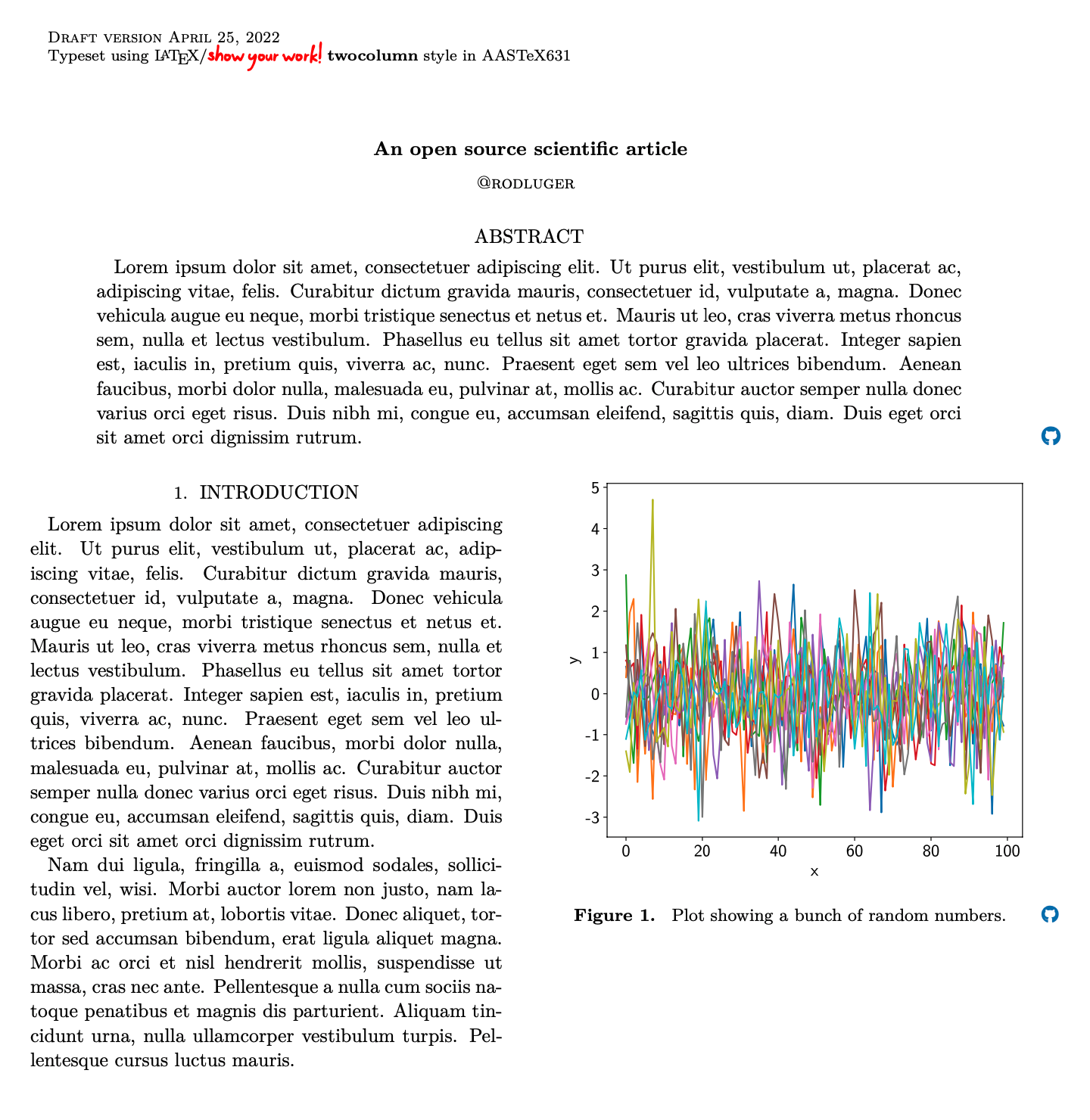
In addition to automatically building our figure for us, showyourwork! has
also included a GitHub icon in the margin next to its caption, which points to
the script that generated it (in this case, random_numbers.py). Importantly,
the link points to the exact version of the script (i.e., to the specific
commit SHA on GitHub) that was used to generate the figure.
If you haven’t yet pushed your changes to GitHub, that URL won’t exist yet; so let’s sync our changes with the remote next.
Build on the remote#
Whenever you make a change to your article (add text, add a figure, edit
a script), make sure to git add any new/modified files,
commit your changes, and then push to the GitHub remote:
git add src/scripts/random_numbers.py
git add src/tex/ms.tex
git commit -m "added a new figure"
git push -u origin main
Note
Note that we’re only adding the figure script, not the figure file, to
the list of files tracked by git. In fact, if you try to add the figure
file, you’ll get an error:
git add src/tex/figures/random_numbers.pdf

The following paths are ignored by one of your .gitignore files:
src/tex/figures/random_numbers.pdf
Use -f if you really want to add them.
As soon as you push your changes to GitHub, a GitHub Action will be triggered
on your repository, which will build your article from scratch on the cloud.
To track the build, click on the  tab of your repository. The first
time your article is built, the action will have to download and install
tab of your repository. The first
time your article is built, the action will have to download and install
conda, so it will likely take a few minutes. Subsequent builds take
advantage of intelligent cross-build caching, so they will likely run
faster.
When the build is done, you can click on any of the badges on the front page of your repository:
these will take you to the build logs, the article tarball (containing the TeX files and all generated figures), and the compiled PDF of the article, respectively.
That’s it for this quickstart tutorial. Please check out the rest of the documentation for more information on how to customize your workflow, debug issues, etc.